2 Animal initial conditions and weekly weights

2.0.1 Downloads

The downloads for this chapter are:

• Data collection template for collecting initial information about the experimental animals and regular weight measurements, cage changes, and adverse events throughout the experiment
• Report template to process data collected with the template (when you go to this link, go to the “File” bar in your browser’s menu bar, chose “Save As”, then save the file as “animal_weights.Rmd”)
• Example output from the report template

2.0.2 Overview

We use the template in this section to record information about each animal used in the experiment. This includes the species, sex, and experimental group. It also includes some information to identify the animal, which in the case of mice includes a code describing the pattern of notches put in the mouse’s ear and the cage that the animal is assigned to at the beginning of the experiment. These are all values that can be determined at the start of the experiment, when the mice are first assigned to groups.

This template is also used to record some data over the course of the experiment. This includes adverse events and cases where an animal is moved from one cage to another during the experiment.

In addition, in our experiments, we are measuring the mice every week to record their weight over the course of the experiment. This weight measuring begins before the first vaccination and continues through until the last mouse is sacrificed. We have used ear notches to identify each mouse, and between the ear notch and the mouse’s cage number, we can uniquely track each mouse in the study.

There are a few reasons that we are measuring these mouse weights. The first is to help us manage the mice, particularly in terms of animal welfare. If there are mice that are losing a lot of weight, that can be an indication that they may need to be euthanized. For example, some animal care standards consider that an adult animal that has lost 20% or more of its weight compared to its baseline weight is indicating a clear sign of morbidity or suffering.

A second reason is that the weight measure might provide a record of each mouse’s general health over the course of the study. In the study, mice are weighed in grams weekly to monitor clinical status, as one potential sign of tuberculosis infection and severity is weight loss.

In humans, tuberculosis patients frequently display weight loss as a clinical symptom associated with disease progression. In particular, extreme weight loss and loss of muscle mass, also known as cachexia, can present as a result of chronic inflammatory illnesses like tuberculosis (Baazim, Antonio-Herrera, and Bergthaler 2022). This cachexia is part of a systemic response to inflammation, and in humans has been linked to upregulation of pro-inflammatory cytokines including tumor necrosis factor, interleukin-6, and interferon-gamma (Baazim, Antonio-Herrera, and Bergthaler 2022). Additionally, studies support a role in cachexia of key immune cell populations such as cytotoxic T-cells which, when depleted, counteract muscle and fat deterioration (Baazim et al. 2019), suggest that thsi type of T-cells may metabolically reprogram adipose tissue.

Given these relationships between weight loss, diseases, and immune processes, it is possible that mouse weight might provide a regularly measurable insight into the severity of disease in each animal. While many of data points are collected to measure the final disease state of each animal, fewer are available before the animal is sacrificed. We are hoping that mouse weights will provide one measure that, while it may not perfectly capture disease severity, may provide some information throughout the experiment that is correlated to disease severity at regular time intervals.

Other studies that use a mouse model of tuberculosis have collected mouse weights, as well (Smith et al. 2022; Segueni et al. 2016). We plan to investigate these data to visualize the trajectory of weight gain / loss in each mouse both before and after they are challenged with tuberculosis. We also plan to test whether each mouse’s weight change after challenge is correlated with other metrics of the severity of disease and immune response. We will do this by testing the correlation between the percent change in weight between challenge and sacrifice with CFUs at sacrifice as well as expression of cytokines and other biological markers (Smith et al. 2022).

2.0.3 Template description

Both the animals’ initial conditions and their weekly measures (adverse events, cage changes, and weights) should be recorded in an excel worksheet. You can download a copy of the template here.

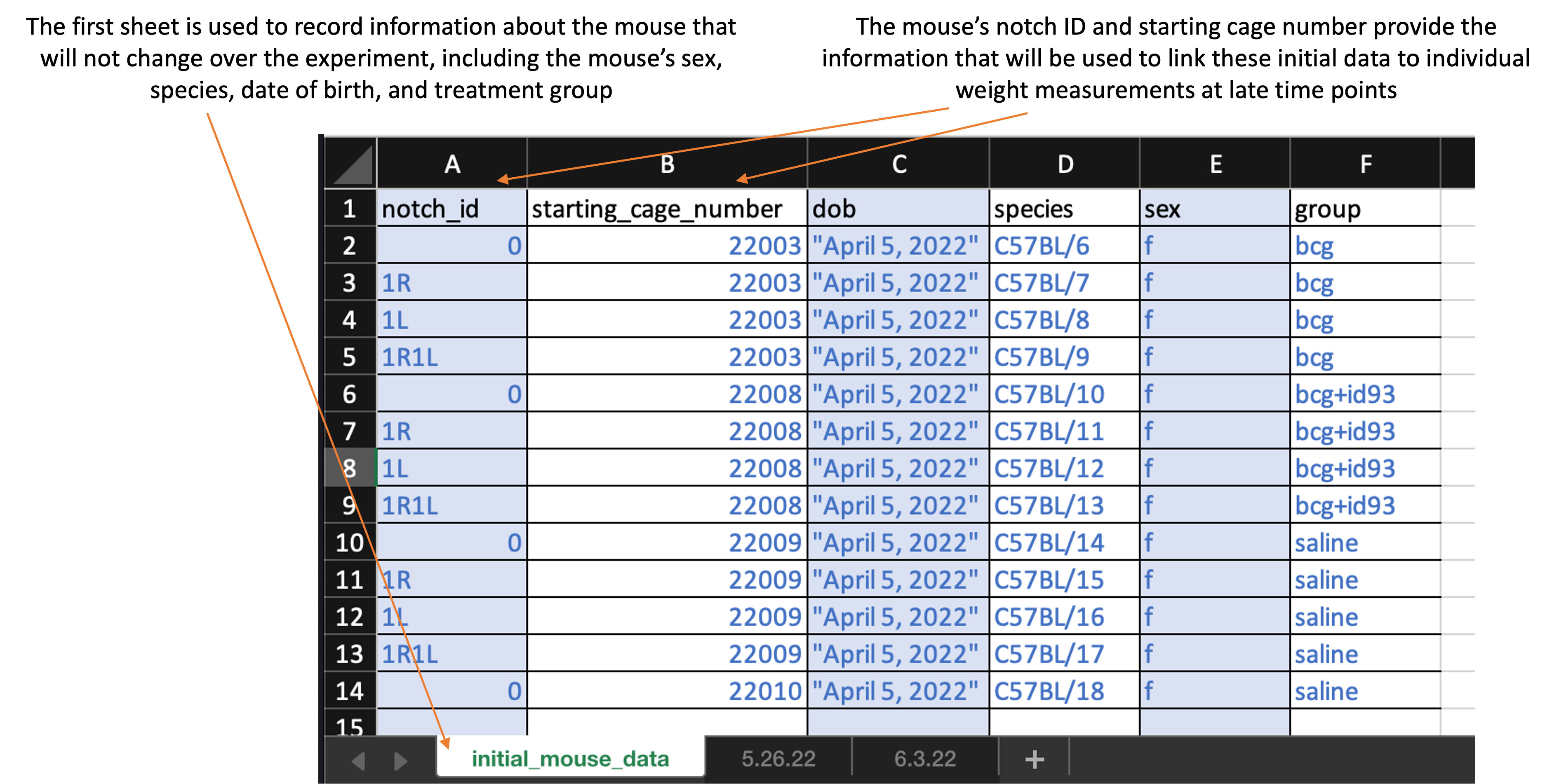
The worksheet is divided into sheets. The first sheet is recorded at the first time point when the mice are measured and is used to record information about the mice that will remain unchanged over the course of the study, like species and sex. Here is what the first sheet of the template looks like:

The second and later sheets are used to record the weight at each measured timepoint. The second sheet will record the weights on the first date they are measured, so it should be recorded at the same time as the first sheet—with initial mouse information—is completed. Here is what the first sheet of the template looks like:

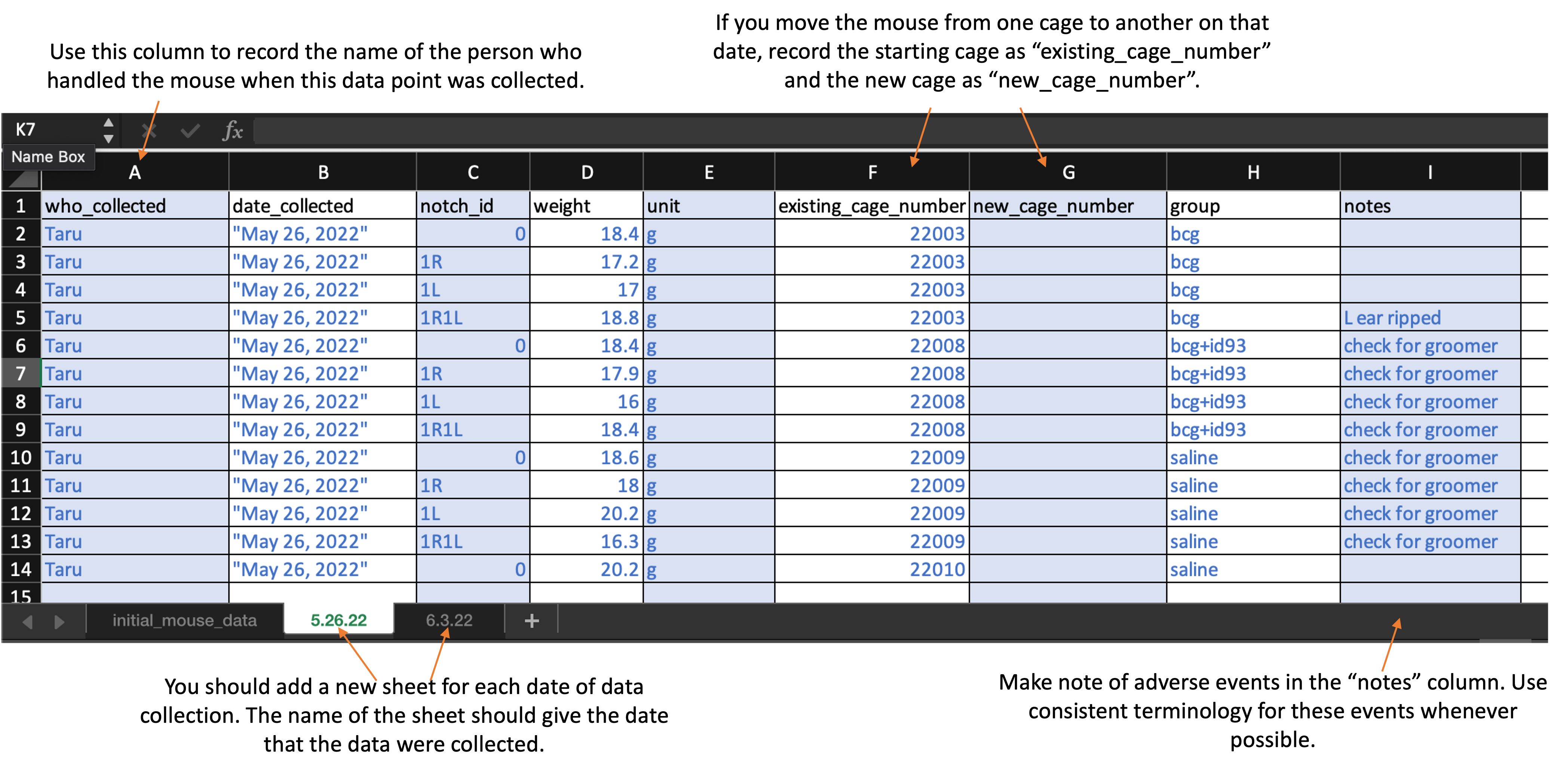
As you continue to measure at new timepoints, you should add a sheet at each timepoint, with each new sheet following the format of the second sheet in the template. The second and later sheets should be labeled with the date when those weights were measured (e.g., “5.26.22” for weights measured on May 26, 2022).

When you download the template, it will have example values filled out in blue. Use these to get an idea for how to record your own data. When you are ready to record your own data, delete these example values and replace them with data collected from your own experiment.

Column titles are as follows. First, in the first sheet, you will record:

• notch_id: Record the ear notch pattern in the mouse. Make sure that you record consistently across all timepoints, so that each mouse can be tracked across dates. If you are doing single notches, for example, this might be “0” for no notches, “1R” for one notch in the right ear, “1L” for one notch in the left ear, and “1R1L” for one notch in each ear.
• starting_cage_number: Record the number of the cage that the mouse is put into at the start of the experiment. In combination with the mouse’s notch_id, this will provide a unique identifier for each mouse at the start of the experiment.
• dob: Record the date the mouse was born.
• species: Record the species of the mouse (e.g., “C57BL/6” for C57 black 6 mice or “CBA” for CBA mice).
• sex: Record as “m” for male or “f” for female
• group: Provide the experimental group of the mouse. Be sure that you use the same abbreviation or notation across each timepoint. Examples of group designations might be: bcg, saline, bcg+id93, saline+id93, saline+noMtb

For the second and later sheets, you will record:

• who_collected: Record the first name of the person who actually handled the mouse from the scale.
• date_collected: Record the date using quotation marks, with the month, then day, then year. For example, “May 31, 2022”.
• weight: Record as a number, without a unit in this column. The next column will be used for the units.
  
• unit: Provide the units that were used to take the weight (e.g., “g” for grams). Be consistent across all animals and timepoints in the abbreviation that you use (e.g., always use “g” for grams, not “g” sometimes and “grams” sometimes)
• existing_cage_number: Provide the cage number that the mouse is in when you start weighing at that time point. If the mouse is moved to another cage on this day, you will specify that in the next column. If the animal was moved from one cage to another between the last weighing and the date of the timepoint you are measuring, put in this column the cage number that the animal was in the last time it was weighed.
• new_cage_number: If the animal is moved to a new cage on the date of the timepoint you are measuring, then use this column to record the number of the cage you move it too. Similarly, if the animal moved cages between the last measured timepoint and this one, use this column to record the cage it was moved to. Otherwise, if the animal stays in the same cage that it was at the last measured time point, leave this column empty.
• group: Provide the experimental group of the mouse. Be sure that you use the same abbreviation or notation across each timepoint. Examples of group designations might be: bcg, saline, bcg+id93, saline+id93, saline+noMtb
• notes: Record information regarding clinical observations (e.g., “back is balding”, “barbering”, “excessive grooming”, “euthanized”).

2.0.4 Processing collected data

Once data are collected, the file can be run through an R workflow. This workflow will convert the data into a format that is easier to work with for data analysis and visualization. It will also produce a report on the data in the spreadsheet, and ultimately it will also write relevant results in a format that can be used to populate a global database for all experiments in the project.

The next section provides the details of the pipeline. It aims to explain the code that processes the data and generates visualizations. You do not need to run this code step-by-step, but instead can access a script with the full code here.

To use this reporting template, you need to download it to your computer and save it in the file directory where you saved the data you collected with the data collection template. You can then open RStudio and navigate so that you are working within this directory. You should also make sure that you have installed a few required packages on R on the computer you are using to run the report. These packages are: tidyverse, purrr, lubridate, readxl, knitr, and ggbeeswarm.

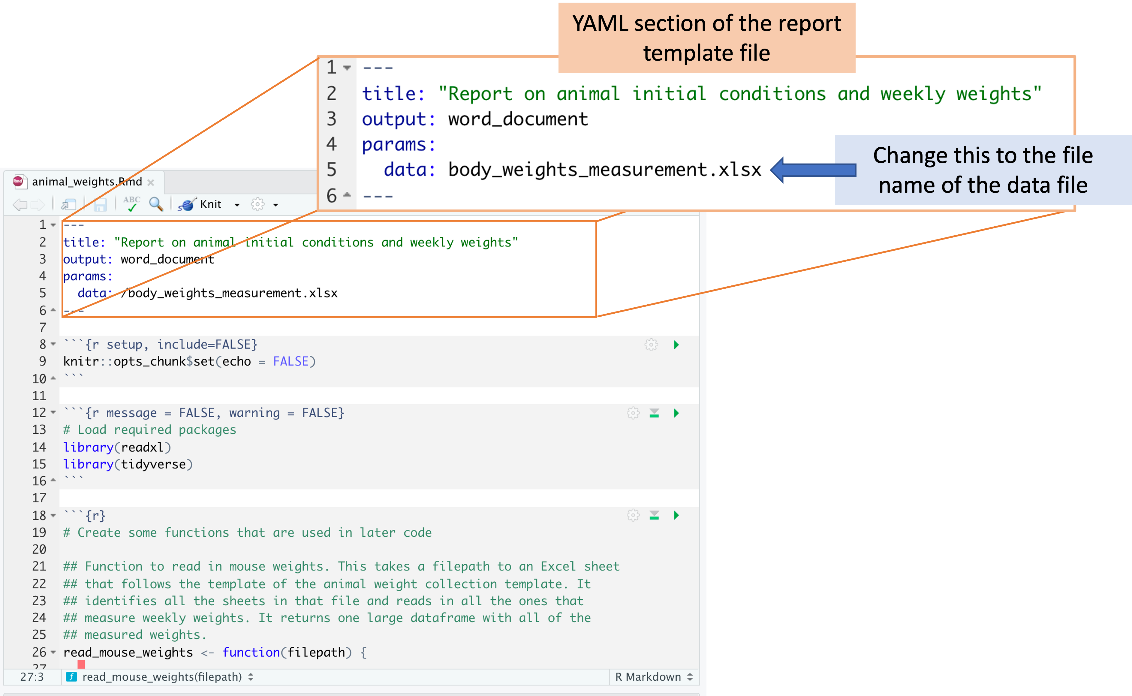
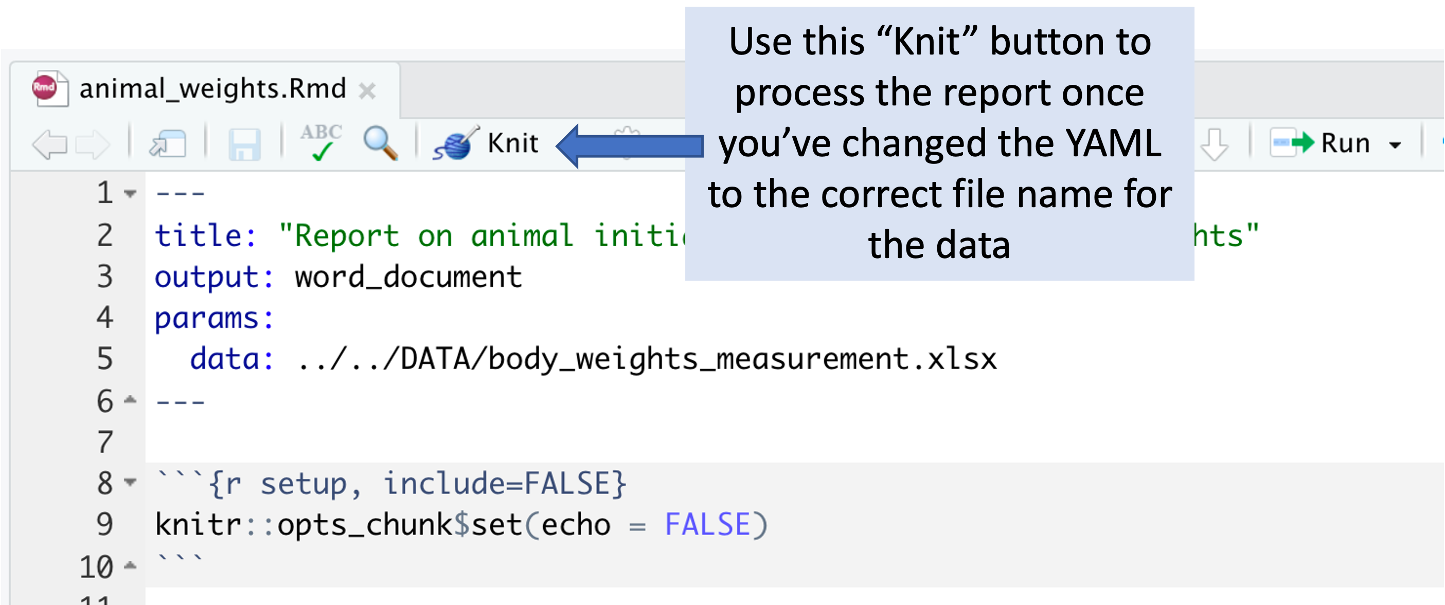
Within RStudio, open the report template file. There is one spot where you will need to change the code in the template file, so it will read in the data from the version of the template that you saved, which you may have renamed. In the YAML of the report template file, change the file path beside “data:” so that it is the file name of your data file.

Once you’ve made this change, you can use the “Knit” button in RStudio to create a report from the data file and the report template file.

The report includes the following elements:

• Summary table of animals at the start of the experiment
• Time series plots of animal weights over the experiment, grouped by experimental group
• Boxplots of the distribution of animal weights within each experimental group at the last available time point
• Plot of measured weight, identified by the person who was handling the animal, to help determine if there are consistent differences by handler
• Table of all the animals in the experiment at the last measured time point, ordered by their weight change since the previous measurement. This table is meant to help in identifying animals that may need to be euthanized for animal welfare reasons.

You can download an example of a report created using this template by clicking here.

When you knit to create the report, it will create a Word file in the same file directory where you put your data file and report template. It will also create and output a version of the data that has been processed (in the case of the weights data, this mainly involves tracking mice as they change cages, to link all weights that are from a single animal). This output fill will be named “mouse_weights_output.csv” and, like the report file, will be saved in the same file directory as the data file and the report template.

2.0.5 Details of processing script

This section goes through the code within the report template. It explains each part of the code in detail. You do not need to understand these details to use the report template. However, if you have questions about how the data are being processed, or how the outputs are created, all those details are available in this section.

As a note, there are two places in the following code where there’s a small change compared to the report template. In the report, you incorporate the path to the data file using the data: section in the YAML at the top of the document. In the following code, we’ve instead used the path of some example data within this book’s file directory, so the code will run for this chapter as well.

First, the workflow loads some additional R libraries. You may need to install these on your local R session if you do not already have them installed.

library(readxl)
library(tidyverse)
library(ggbeeswarm)

These packages bring in some useful functions that are not available in the base installation of R. They are all open source. To cite any of them, you can use the citation function. For example, to get the information you would need to cite the readxl package, in R you can run:

citation("readxl")

## To cite package 'readxl' in publications use:
## 
##   Wickham H, Bryan J (2023). _readxl: Read Excel Files_. R package
##   version 1.4.3, <https://CRAN.R-project.org/package=readxl>.
## 
## A BibTeX entry for LaTeX users is
## 
##   @Manual{,
##     title = {readxl: Read Excel Files},
##     author = {Hadley Wickham and Jennifer Bryan},
##     year = {2023},
##     note = {R package version 1.4.3},
##     url = {https://CRAN.R-project.org/package=readxl},
##   }

Next, the code in the report template creates a few custom functions to help process the data from the data collection template. The first of these functions checks the data collection template to identify all the timepoints that were collected and then reads each in, ultimately joining data from all time points into one large dataset.

The data collection template requires you to use a new sheet in the spreadsheet for each weight collection time point, with a first sheet that records initial information about the animals. If you only take weights at three time points, there would only be three time point sheets in the final file. Conversely, if you collect weight data at twenty time points, there would be twenty sheets in the final file. The first function, called ``, reads the data file, checks to find all the weight recording sheets, whether it’s three or twenty, and then reads the data in from all the sheets and binds them together into a single dataframe.

## Function to read in mouse weights. This takes a filepath to an Excel sheet
## that follows the template of the animal weight collection template. It 
## identifies all the sheets in that file and reads in all the ones that 
## measure weekly weights. It returns one large dataframe with all of the 
## measured weights. 
read_mouse_weights <- function(filepath) {
  
  # getting info about all excel sheets
  mouse_weights_sheets <- readxl::excel_sheets(filepath)[-1] # First sheet is initial data, not mouse weights
  
  mouse_weights <- purrr::map(mouse_weights_sheets, 
                              ~ readxl::read_excel(filepath, sheet = .x, 
                                                   col_types = c("text",   # who_collected
                                                                 "text",   # date_collected
                                                                 "text",   # notch_id
                                                                 "numeric", # weight
                                                                 "text",   # unit
                                                                 "text",   # existing_cage_number
                                                                 "text",   # new_cage_number
                                                                 "text",   # group
                                                                 "text"    # notes
                                                                 ))) %>% 
    dplyr::bind_rows() %>% 
    mutate(date_collected = lubridate::mdy(date_collected))

  return(mouse_weights)
}

The remaining functions are all functions to help track a mouse over the experiment even if it changes cages. In processing this data, the key challenge is to track a single mouse over the experiment. The mice are identified by a pattern of notches in their ears. However, there are a limited number of notches that can be distinguished, so the notch information does not distinctly identify every mouse in the study, just every mouse within a certain cage. By knowing both an ear notch ID and a cage number, you can distinctly identify each mouse in the study.

However, mice are moved from one cage to another in some cases during a study. If mice within a cage are fighting, or if they are showing signs of excessive grooming, these can be reasons to move a mouse to a new cage once the experiment has started. The cage moves need to be resolved when processing the data so that each mouse can be tracked even as they move.

In the data collection template, we have created a design that aims to include information about cage moves, but to do so in a way that is as simple as possible for the person who is recording the data. The weights are recorded for each time point in a separate sheet of the data collection template. On the sheet for a time point, there are also columns to give the mouse’s cage at the start of that data collection time point, as well as the cage the mouse was moved to, if it was moved. The report template code then uses this information to create a unique ID for each mouse (one that is constant across the experiment), and then attach it to the mouse’s measurements even as the mouse is moved from one cage to another. The following two functions both help with this process:

# Function to get the next cage number based on the 
# existing cage number and notch ID. If the mouse does not
# switch cages again, the output is a vector of length 0. 
# This takes the dataframe and existing identifiers (notch id and
# existing cage number) as inputs. It returns the next cage
# that the mouse was moved to. If the mouse has not moved
# from the existing case, the output has length 0.
get_next_cage <- function(existing_cage_number, notch_id, 
                          df = our_mouse_weights){
  next_cage <- df %>% 
    filter(.data$existing_cage_number == {{existing_cage_number}} &
             .data$notch_id == {{notch_id}} & 
             !is.na(.data$new_cage_number)) %>% 
    pull(new_cage_number)
  
  return(next_cage)
}

# Function to get the full list of cages for each individual 
# mouse, over the course of all data collected to date. This 
# inputs the starting identifiers of the mouse (starting cage ID 
# and notch ID). It then works through any cage changes to create
# a list for that mouse of all cages it was put in over the 
# course of the experiment. 
get_mouse_cages <- function(mouse_starting_cage, mouse_notch_id, 
                            df = our_mouse_weights){
  mouse_cage_list <- mouse_starting_cage
  i <- 1
  
  while(TRUE){
    next_cage <- get_next_cage(existing_cage_number =
                               mouse_cage_list[i],
                               notch_id = mouse_notch_id, 
                               df = df)
    if(length(next_cage) == 0) {
      break
      }
    i <- i + 1
    mouse_cage_list[i] <- next_cage
    }
  
  return(mouse_cage_list)
}

Next, the report template code gets to the workflow itself, where it uses both these custom functions and other R code to process the data and then to provide summaries and visualizations of the data.

The first step in the workflow is to read in the data from the spreadsheet. As long as the data are collected following the template that was described earlier, this code should be able to read it in correctly and create a master dataset with the data from all sheets of the spreadsheet. This step of the pipeline uses one of the custom functions that was defined at the start of the report template code:

# Read in the mouse weights from the Excel template. This creates one large
# dataframe with the weights from all the timepoints. 
our_mouse_weights <- read_mouse_weights(filepath =
                                          "DATA/body_weights_measurement.xlsx")

Next, the code runs through a number of steps to create a unique ID for each mouse and then apply that ID to each time point, even if a mouse changes cages.

# Add a unique mouse ID for the first time point. This will become each mouse's
# unique ID across all measured timepoints.
our_mouse_weights <- our_mouse_weights %>% 
  mutate(mouse_id = 1:n(), 
         mouse_id = ifelse(date_collected ==
                                    first(date_collected), 
                                  mouse_id, 
                                  NA))

# Create a dataframe that lists all mice at the first time point, 
# as well as a list of all the cages they have been in over the
# experiment
mice_cage_lists <- our_mouse_weights %>% 
  filter(date_collected == first(date_collected)) %>% 
  select(notch_id, existing_cage_number, mouse_id) %>% 
  mutate(cage_list = map2(.x = existing_cage_number, 
                          .y = notch_id, 
                          .f = ~ get_mouse_cages(.x, .y, df = our_mouse_weights)))

# Add a column with the latest cage to the weight dataframe
our_mouse_weights$latest_cage <- NA

# Loop through all the individual mice, based on mice with a 
# measurement at the first time point. Add the unique ID for 
# each mouse, which will apply throughout the experiment. Also 
# add the most recent cage ID, so the mouse can be identified
# by lab members based on it's current location
for(i in 1:nrow(mice_cage_lists)){
  this_notch_id <- mice_cage_lists[i, ]$notch_id
  this_cage_list <- mice_cage_lists[i, ]$cage_list[[1]]
  this_unique_id <- mice_cage_lists[i, ]$mouse_id
  latest_cage <- this_cage_list[length(this_cage_list)]
  
  our_mouse_weights$mouse_id[our_mouse_weights$notch_id == this_notch_id & 
                       our_mouse_weights$existing_cage_number %in% 
                       this_cage_list] <- this_unique_id
  
  our_mouse_weights$latest_cage[our_mouse_weights$notch_id == this_notch_id & 
                       our_mouse_weights$existing_cage_number %in% 
                       this_cage_list] <- latest_cage
}

# Add a label for each mouse based on its notch_id and latest cage
our_mouse_weights <- our_mouse_weights %>% 
  mutate(mouse_label = paste("Cage:", latest_cage, 
                             "Notch:", notch_id))

Ultimately, this creates both a unique ID for each mouse (in a column of the dataframe called mouse_id), as well as creates a unique label that can be used in plots and tables (given in the mouse_label column). The unique ID is set at the beginning of the study for each mouse and remains the same throughout the study. The label, on the other hand, is based on the mouse’s ear notch pattern and the most recent cage it was recorded to be in. We made this choice for a labeling identifier, because it will help the researchers to quickly identify a mouse in the study based on it’s current, rather than starting, cage.

The next part of the code reads in the initial data that were recorded for each animal in the experiment. The code then pulls in information from the processed weights dataset to match these initial data with each animals unique ID. Ultimately, these starting data are incorporated into the large dataset of mouse weights, creating a single large dataset to work with (our_mouse_weights) that includes all the information that was recorded in the data collection template.

# Read in the data from the original file with the initial animal 
# characteristics
mouse_initial <- readxl::read_excel("DATA/body_weights_measurement.xlsx", 
                                      sheet = 1, 
                                      col_types = c("text", # notch_id
                                                    "text", # starting_cage_number
                                                    "text", # dob
                                                    "text", # species
                                                    "text", # sex
                                                    "text" # group
                                                    )) %>%
  mutate(dob = lubridate::mdy(dob), 
         sex = forcats::as_factor(sex))

# Figure out the starting cage for each mouse, so they can be incorporated
# with the initial data so we can get the mouse ID that was added for the 
# starting time point
mouse_ids <- our_mouse_weights %>% 
  filter(date_collected == first(date_collected)) %>% 
  select(notch_id, existing_cage_number, mouse_id) %>% 
  rename(starting_cage_number = existing_cage_number)

# Merge in the mouse IDs with the dataframe of initial mouse characteristics
mouse_initial <- mouse_initial %>% 
  left_join(mouse_ids, by = c("notch_id", "starting_cage_number"))

# Join the initial data with the weekly weights data into one large dataset
our_mouse_weights <- our_mouse_weights %>% 
  left_join(mouse_initial, by = c("mouse_id", "notch_id", "group"))

At this point, the first few rows of this large dataset look like this:

our_mouse_weights %>% 
  slice(1:5)

## # A tibble: 5 × 16
##   who_collected date_collected notch_id weight unit  existing_cage_number
##   <chr>         <date>         <chr>     <dbl> <chr> <chr>               
## 1 Taru          2022-05-26     0          18.4 g     22003               
## 2 Taru          2022-05-26     1R         17.2 g     22003               
## 3 Taru          2022-05-26     1L         17   g     22003               
## 4 Taru          2022-05-26     1R1L       18.8 g     22003               
## 5 Taru          2022-05-26     0          18.4 g     22004               
## # ℹ 10 more variables: new_cage_number <chr>, group <chr>, notes <chr>,
## #   mouse_id <int>, latest_cage <chr>, mouse_label <chr>,
## #   starting_cage_number <chr>, dob <date>, species <chr>, sex <fct>

The rest of the code in the report template will create summaries and graphs of the data. First, there is some code that provides summaries of the research animals at the start of the experiment. It uses the mouse_initial dataset (which pulled in data from the first sheet of the data collection template). It uses a summarize call to summarize details from this sheet of data, including the species of the animal, the total number of animals, how many were males versus females, and which experimental groups were included. It uses some additional code to format the data so the resulting table will be clearer, and then uses the kable function to output the results as a nicely formatted table.

# Create a table that summarizes the animals at the start of the experiment
mouse_initial %>% 
  summarize(Species = paste(unique(species), collapse = ", "), 
            `Total animals` = n(), 
            `Sex distribution` = paste0("male: ", sum(sex == "m"), 
                                      ", female: ", sum(sex == "f")),
            `Experimental groups` = paste(unique(group), collapse = ", "),
            `N. of starting cages` =
              length(unique(starting_cage_number))) %>% 
  mutate_all(as.character) %>% 
  pivot_longer(everything()) %>% 
  mutate(name = paste0(name, ":")) %>% 
  knitr::kable(col.names = c("", ""), 
               caption = "Summary of experimental animals at the start of the experiment", 
               align = c("r", "l"))

Table 2.1: Summary of experimental animals at the start of the experiment

Species:	C57BL/6
Total animals:	140
Sex distribution:	male: 60, female: 80
Experimental groups:	bcg, bcg+id93, saline, saline+id93, saline+noMtb
N. of starting cages:	34

The next piece of code creates a time series of mouse weights over time. The points for each mouse are connected to create a line, so it’s easy to see both variation across mice at a single time point and variation in a single mouse over the study. The lines are colored to distinguish male from female mouse (and there is a clear difference in average weights in the two groups). The plot is faceted so that the time series for mice in each experimental group are shown in different small “facets” of the plot, but with the same axis ranges used on each small plot to help comparisons across plots.

# Create a plot of mouse weights over time
our_mouse_weights %>% 
  ggplot(aes(x = date_collected, y = weight, 
             group = mouse_id, color = sex)) + 
  geom_line() + 
  facet_wrap(~ group) + 
  ggtitle("Animal weights over time by experiment group") +
  labs(x = "Date collected", 
       y = "Weight (g)")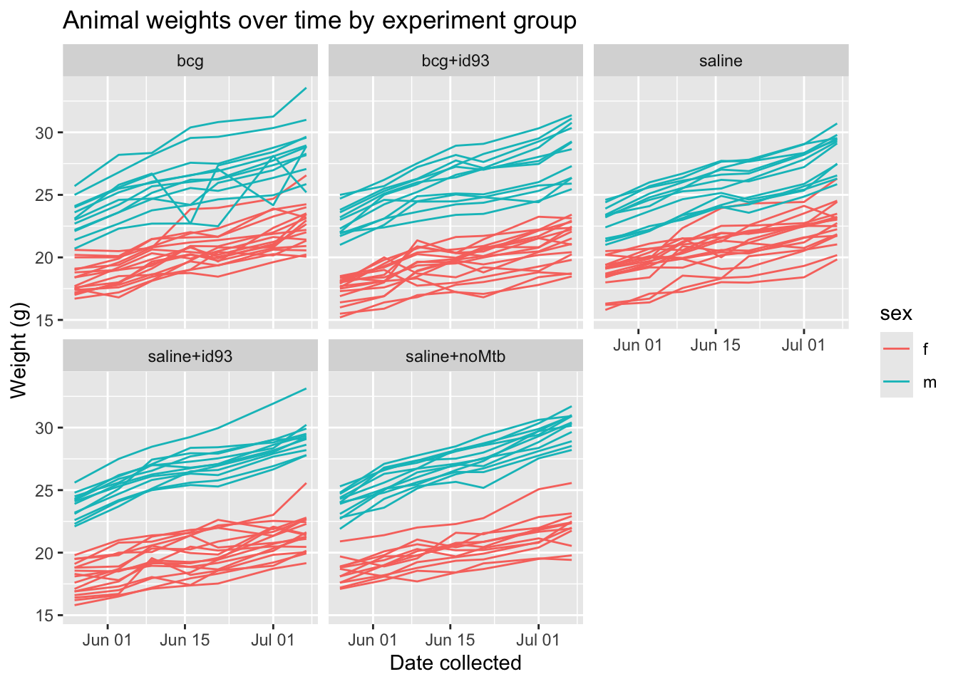

Next, the code creates boxplots that focus on differences in weights at the latest available timepoint. One boxplot is created for each experimental group, and the points for individual mice are shown behind the boxplot, to provide a better idea of the pattern of variation in individual mice. These points are colored based on sex, to help explore patterns by sex.

# Plot animal weight boxplots for the latest time point 
our_mouse_weights %>% 
  filter(date_collected == last(date_collected)) %>% 
  ggplot(aes(x = group, y = weight)) + 
  geom_beeswarm(aes(color = sex)) + 
  geom_boxplot(fill = NA, color = "dodgerblue") + 
  ggtitle("Animal weights at last collection by experimental group") + 
  labs(x = "Experimental group", 
       y = "Weight (g)")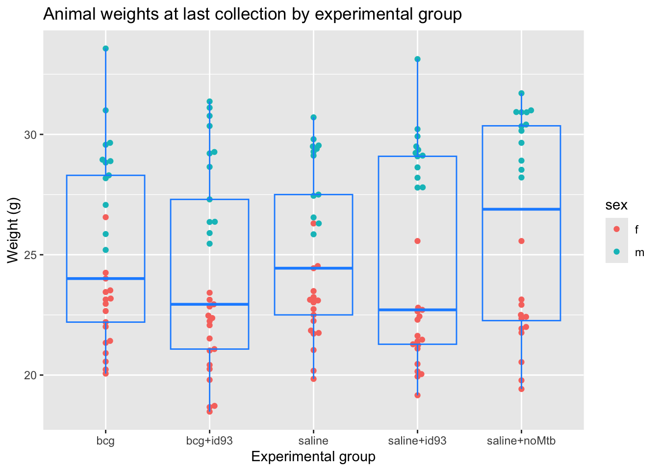

The next piece of code shows how mouse weights vary by the person who was handling the animals at a certain time point. Different handlers may have small differences in how they handle and weight the mice. If there are noticable differences in the measured weights, this is something that could be corrected through statisical modeling in later analysis, so we included it as a potential check.

# Plot animal weights by animal handler
our_mouse_weights %>% 
  ggplot(aes(x = date_collected, y = weight, color = who_collected)) + 
  geom_point() + 
  ggtitle("Animal weights by animal handler") + 
  labs(x = "Date collected", 
       y = "Weight (g)",
       color = "Person who\nhandled the\nanimal")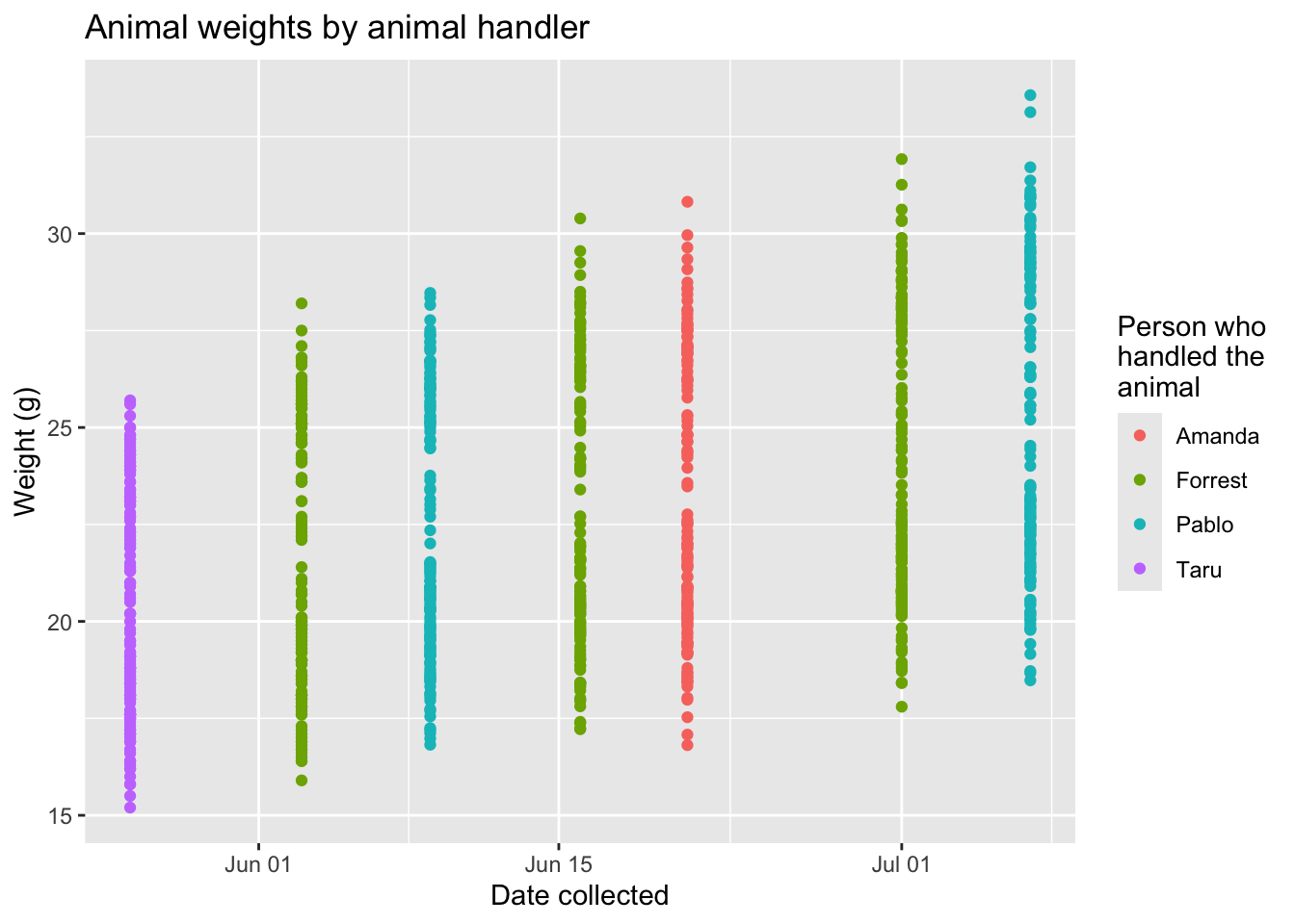

The next piece of code creates a table with each of the animals that was still tracked at the last time point (if animals were sacrificed prior to the last recorded time point, they would not be included here). This table focuses on the weight change since the previous measured time point. It is ordered by the change in weight, from the largest decrease to the largest increase. It is meant as an aide in identifying mice that are showing signs of suffering and may need to be considered for being euthanized. The animals are labeled in this table by their most recent cage location, so it will be easier to find them if necessary. For this example code, we’ve shown only a sample of 15 animals, but the report will show data for all animals.

# Create table of animal weight changes since previous time point
our_mouse_weights %>% 
  select(date_collected, weight, group, mouse_label, sex) %>% 
  group_by(mouse_label) %>% 
  mutate(weight_change = (weight - lag(weight)) / lag(weight)) %>% 
  ungroup() %>% 
  filter(date_collected == last(date_collected)) %>% 
  mutate(formatted_weight_change = paste0(formatC(weight_change * 100, 
                                                  digits = 1, format = "f"), "%")) %>% 
  arrange(weight_change) %>% 
  select(mouse_label, group, sex, weight, formatted_weight_change) %>% 
  slice(1:15) %>%  # Only for the chapter--show a sample, not all
  knitr::kable(col.names = c("Mouse", "Experimental group", "Sex", 
                             "Weight (g)", "Weight change since last measure"), 
               caption = "Individual data on weight changes in mice between current measurement and previous measurement.")

Table 2.2: Individual data on weight changes in mice between current measurement and previous measurement.

Mouse	Experimental group	Sex	Weight (g)	Weight change since last measure
Cage: 22021 Notch: 1R	bcg	m	25.20	-10.4%
Cage: 22017 Notch: 1R	saline	f	23.13	-4.1%
Cage: 22015 Notch: 1L	bcg	f	23.18	-3.1%
Cage: 22476 Notch: 1R1L	saline+noMtb	f	20.54	-2.8%
Cage: 22014 Notch: 1L	saline+id93	f	21.47	-2.8%
Cage: 22014 Notch: 0	saline+id93	f	21.40	-2.7%
Cage: 22006 Notch: 1R1L	bcg+id93	f	21.02	-2.4%
Cage: 22015 Notch: 0	bcg	f	20.06	-1.0%
Cage: 22004 Notch: 1R	bcg	f	21.42	-1.0%
Cage: 22006 Notch: 0	bcg+id93	f	18.67	-0.7%
Cage: 22476 Notch: 0	saline+noMtb	f	19.42	-0.6%
Cage: 22016 Notch: 1R1L	bcg+id93	f	23.13	-0.5%
Cage: 22012 Notch: 1R	saline+id93	f	22.44	-0.4%
Cage: 22015 Notch: 2L	bcg	f	20.56	-0.3%
Cage: 22013B Notch: 1L	saline+id93	f	20.46	-0.2%

As a last step, the code in the template writes a CSV file with the processed data. This file will be an input into a script that will format the data to add to a database where we are collecting and integrating data from all the CSU experiments, and ultimately from there into project-wide storage.

# Write out processed data into a CSV file
write_csv(our_mouse_weights, "mouse_weights_output.csv")