3 Colony forming units to determine bacterial counts
3.0.1 Downloads
The downloads for this chapter are:
- Data collection template for recording colony forming units counted on each plate or section of plate in the laboratory
- Report template to process data collected with the data template (when you go to this link, go to the “File” bar in your browser’s menu bar, chose “Save As”, then save the file as “animal_weights.Rmd”)
- Example output from the report template
3.0.2 Overview
In the experiments, we will need to estimate the bacterial load of Mycobacterium tuberculosis in organs—including lungs and spleens—of animals from experiments. These measurements help us assess how well a vaccine has worked in comparison to controls.
We will be estimating bacterial load in an animal organ using the plate count method with serial dilutions. Serial dilutions allow you to create a highly diluted sample without needing a massive amount of diluent: as you increase the dilution one step at a time, you can steadily bring the samples down to lower bacterial loads per volume. This method is common across laboratories that study tuberculosis drug efficacy as a method for estimating bacterial load in animal organs (Franzblau et al. 2012) and is a well-established method across microbiology in general, dating back to Koch in the late 1800s (Wilson 1922; Ben-David and Davidson 2014).
With this method, we homogenize part of the organ, and then create several increasingly dilute samples. Each dilution is then spread on a plate with a medium in which Mycobacterium tuberculosis can grow and left to grow for several weeks at a temperature conducive to Mycobacterium tuberculosis growth. The idea is that individual bacteria from the original sample end up randomly spread across the surface of the plate, and any bacteria that are viable (able to reproduce) will form a new colony that, after a while, you’ll be able to see (Wilson 1922; Goldman and Green 2015). At the end of this incubation period, you can count the number of these colony-forming units (CFUs) on each plate.
To count the number of CFUs, you need a “just right” dilution (and we often won’t know what this is until after plating) to have a countable plate. If you have too high of a dilution (i.e., one with very few viable bacteria), randomness will play a big role in the CFU count, and you’ll estimate the original with more variability, which isn’t ideal. If you have too low of a dilution (i.e., one with lots of viable bacteria), it will be difficult to identify separate colonies, and they may compete for resources. (The pattern you see when the dilution is too low (i.e., too concentrated with bacteria) is called a lawn—colonies merge together).
Once you identify a good dilution for each sample, the CFU count from this dilution can be used to estimate the bacterial load in the animal’s organ. To translate from diluted concentration to original concentration, you do a back-calculation, incorporating both the number of colonies counted at that dilution and how dilute the sample was (Ben-David and Davidson 2014; Goldman and Green 2015).
3.0.3 Template description
The data are collected in a spreadsheet with multiple sheets. The first sheet (named “metadata”) is used to record some metadata for the experiment, while the following sheets are used to record CFUs counts from the plates used for samples from each organ, with one sheet per organ. For example, if you plated data from both the lung and spleen, there would be three sheets in the file: one with the metadata, one with the plate counts for the lung, and one with the plate counts for the spleen.
The first sheet, which is the metadata sheet, is shown below:
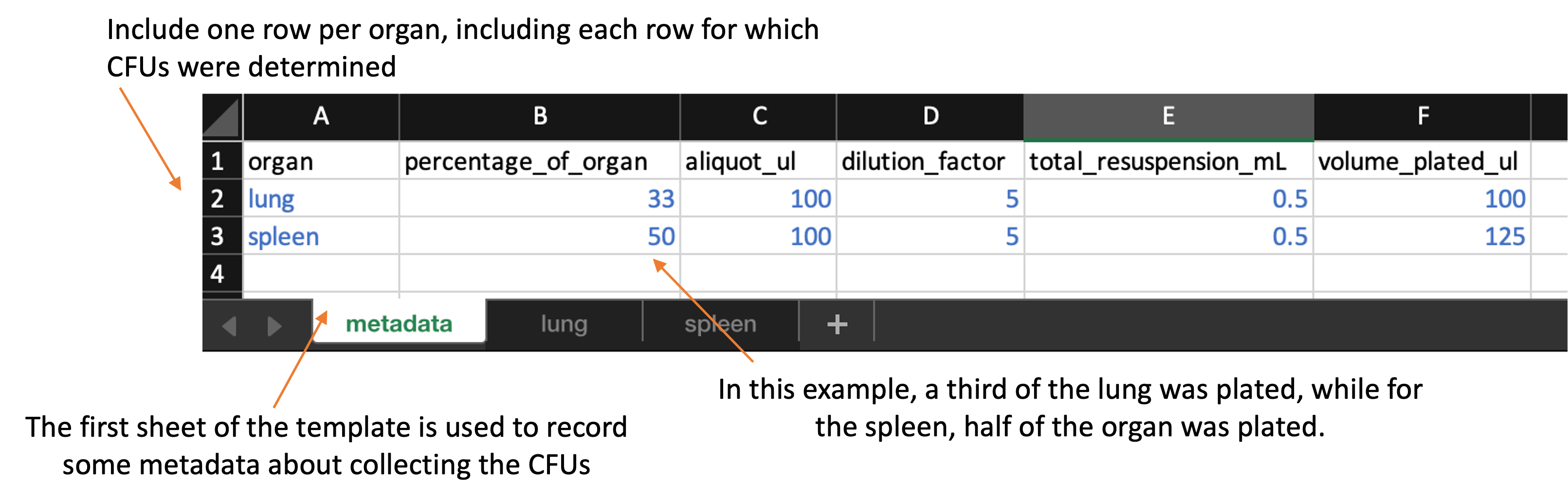
This metadata sheet is used to record information about the overall process of plating the data. Values from this sheet will be used in calculating the bacterial load in the original sample based on the CFU counts. This spreadsheet includes the following columns:
-
organ: Include one row for each organ that was plated in the experiment. You should name the organ all in lowercase (e.g., “lung”, “spleen”). You should use the same name to also name the sheet that records data for that organ for example, if you have rows in the metadata sheet for “lung” and “spleen”, then you should have two other sheets in the file, one sheet named “lung” and one named “spleen”, which you’ll use to store the plate counts for each of those organs. -
percentage_of_organ: In this column, give the proportion of that organ that was plated. For example, if you plated half the lung, then in the “lung” row of this spread sheet, you should put 0.5 in theprop_resuspendedcolumn. -
aliquot_ul: 100 uL of the total_resuspended slurry would be considered an original aliquot and is used to peform serial dilutions. -
dilution_factor: Amount of the original stock solution that is present in the total solution, after dilution(s) -
total_resuspended_mL: This column contains an original volume of tissue homogenate. For example, raw lung tissue is homogenized in 0.5 mL of PBS in a tube containing metal beads. -
volume_plated_ul: Amount of suspension + diluent plated on section of solid agar
Following this first sheet in the file, you should have one sheet for each organ. The organs that you record in these sheets should match up with the rows on the first, metadata sheet of the template.
Each of these organ-specific sheets should look like this:
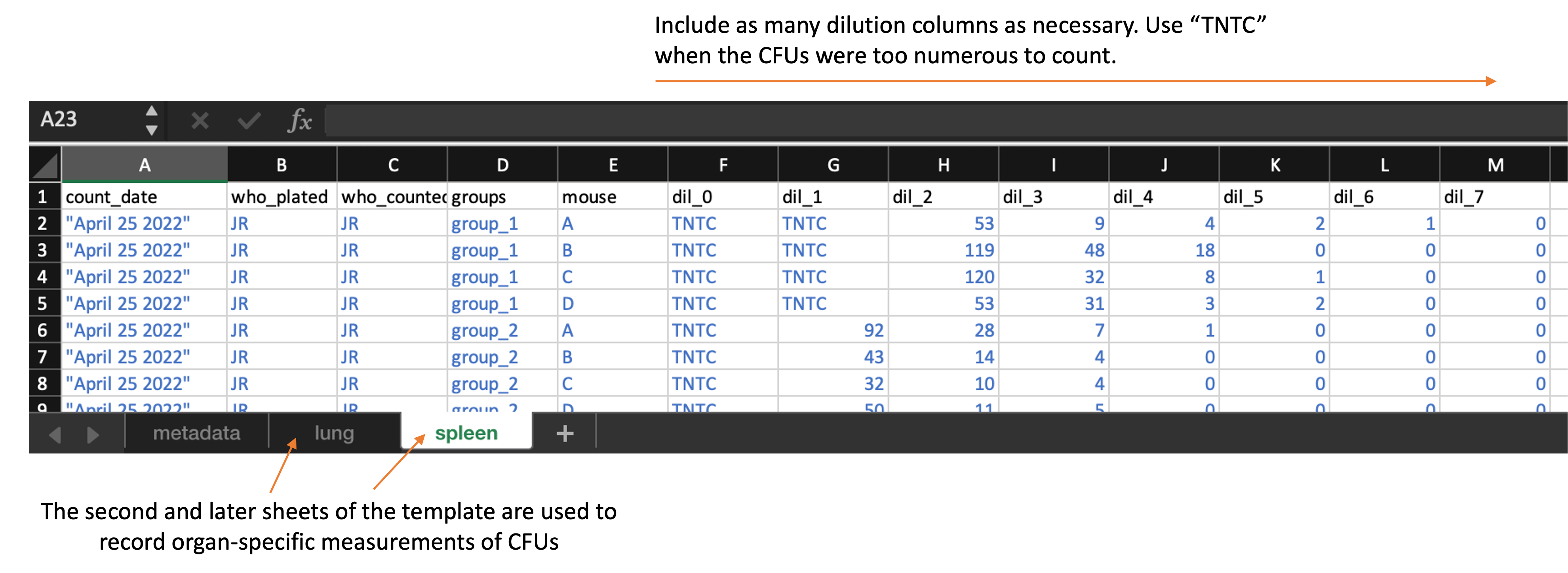
Each of these organ-specific sheets of the template include the following columns:
-
count_date: The date that the CFUs were counted. In some cases, the same plates may be counted at multiple dates. -
who_plated: An identifier for the researcher who plated the sample -
who_counted: An identifier for the researcher who counted the plate on this specific date -
groups: The experimental group to which the mouse belonged to -
mouse: An identifier for the unique mouse within the group (note: as we collect data from the new experiment, this can be a unique ID by mouse, based on notch ID and cage number) -
dil_0,dil_1,dil_2, …: The count at each dilution. You can add additional columns if there were more dilutions that are in the template or take away dilution columns if there were fewer. However, all dilution columns should be named consistently, with “dil_” followed by the dilution number (e.g., “0”, “1”, “2”). If the CFUs were too numerous to count for a sample at a particular dilution, put “TNTC” in that cell of the spreadsheet.
You can download the template here. When you download the template, it will have example values filled out in blue. Use these to get an idea for how to record your own data. When you are ready to record your own data, delete these example values and replace them with data collected from your own experiment.
3.0.4 Processing collected data
Once data are collected, the file can be run through an R workflow. This workflow will convert the data into a format that is easier to work with for data analysis and visualization. It will also produce a report on the data in the spreadsheet, and ultimately it will also write relevant results in a format that can be used to populate a global database for all experiments in the project.
The next section provides the details of the pipeline. It aims to explain the code that processes the data and generates visualizations. You do not need to run this code step-by-step, but instead can access a script with the full code here.
To use this reporting template, you need to download it to your computer and
save it in the file directory where you saved the data you collected with the
data collection template. You can then open RStudio and navigate so that you are
working within this directory. You should also make sure that you have installed
a few required packages on R on the computer you are using to run the report.
These packages are: tidyverse, readxl, ggbeeswarm, ggpubr, purrr,
knitr, and broom.
Within RStudio, open the report template file. There is one spot where you will need to change the code in the template file, so it will read in the data from the version of the template that you saved, which you may have renamed. In the YAML of the report template file, change the file path beside “data:” so that it is the file name of your data file.
Once you’ve made this change, you can use the “Knit” button in RStudio to create a report from the data file and the report template file.
The report includes the following elements:
- Organ-specific summaries of the experiment, including the number of mice, experimental groups, date counted, and dilutions used for each experiment
- Metadata on the CFU collection process (e.g., percent of organ plated for each organ, dilution factor)
- Plot showing the distribution of CFUs by group in each organ
- Table giving the results of an ANOVA analysis comparing log CFUs across groups within each organ
You can download an example of a report created using this template by clicking here.
When you knit to create the report, it will create a Word file in the same file directory where you put your data file and report template. It will also create and output a version of the data that has been processed (in the case of the weights data, this mainly involves tracking mice as they change cages, to link all weights that are from a single animal). This output fill will be named “cfu_output.csv” and, like the report file, will be saved in the same file directory as the data file and the report template.
3.0.5 Details of processing script
This section goes through the code within the report template. It explains each part of the code in detail. You do not need to understand these details to use the report template. However, if you have questions about how the data are being processed, or how the outputs are created, all those details are available in this section.
As a note, there are two places in the following code where there’s a small
change compared to the report template. In the report, you incorporate the path
to the data file using the data: section in the YAML at the top of the
document. In the following code, we’ve instead used the path of some example
data within this book’s file directory, so the code will run for this chapter as
well.
First, the workflow loads some additional R libraries. You may need to install these on your local R session if you do not already have them installed.
Next, the pipeline reads in the organ-specific data. To do this, it creates a list of all of the sheets that are in the spreadsheet other than the metadata sheet. It then loops through each of these organ-specific sheets. It uses pivoting to convert all the dilution levels and values into two columns (a longer rather than wider format), so that the data from all the organs can be joined into a single large dataframe, even if a different number of dilutions were used for the different organs.
## [[1]]
## # A tibble: 880 × 10
##    count_date      who_plated who_counted group mouse day   sex   organ dilution
##    <chr>           <chr>      <chr>       <chr> <chr> <chr> <chr> <chr>    <dbl>
##  1 "\"Dec 28 2023… FL         FL          BCG   1     14    fema… lung         0
##  2 "\"Dec 28 2023… FL         FL          BCG   1     14    fema… lung         1
##  3 "\"Dec 28 2023… FL         FL          BCG   1     14    fema… lung         2
##  4 "\"Dec 28 2023… FL         FL          BCG   1     14    fema… lung         3
##  5 "\"Dec 28 2023… FL         FL          BCG   1     14    fema… lung         4
##  6 "\"Dec 28 2023… FL         FL          BCG   1     14    fema… lung         5
##  7 "\"Dec 28 2023… FL         FL          BCG   1     14    fema… lung         6
##  8 "\"Dec 28 2023… FL         FL          BCG   1     14    fema… lung         7
##  9 "\"Dec 28 2023… FL         FL          BCG   1     14    fema… lung         8
## 10 "\"Dec 28 2023… FL         FL          BCG   1     14    fema… lung         9
## # ℹ 870 more rows
## # ℹ 1 more variable: CFUs <chr>
##
## [[2]]
## # A tibble: 870 × 10
##    count_date      who_plated who_counted group mouse day   sex   organ dilution
##    <chr>           <chr>      <chr>       <chr> <chr> <chr> <chr> <chr>    <dbl>
##  1 "\"Dec 28 2023… FL         FL          BCG   1     14    fema… sple…        0
##  2 "\"Dec 28 2023… FL         FL          BCG   1     14    fema… sple…        1
##  3 "\"Dec 28 2023… FL         FL          BCG   1     14    fema… sple…        2
##  4 "\"Dec 28 2023… FL         FL          BCG   1     14    fema… sple…        3
##  5 "\"Dec 28 2023… FL         FL          BCG   1     14    fema… sple…        4
##  6 "\"Dec 28 2023… FL         FL          BCG   1     14    fema… sple…        5
##  7 "\"Dec 28 2023… FL         FL          BCG   1     14    fema… sple…        6
##  8 "\"Dec 28 2023… FL         FL          BCG   1     14    fema… sple…        7
##  9 "\"Dec 28 2023… FL         FL          BCG   1     14    fema… sple…        8
## 10 "\"Dec 28 2023… FL         FL          BCG   1     14    fema… sple…        9
## # ℹ 860 more rows
## # ℹ 1 more variable: CFUs <chr>
## # A tibble: 6 × 10
## count_date who_plated who_counted group mouse day sex organ dilution CFUs
## <chr> <chr> <chr> <chr> <chr> <chr> <chr> <chr> <dbl> <chr>
## 1 "\"Dec 28… FL FL BCG 1 14 fema… lung 0 TNTC
## 2 "\"Dec 28… FL FL BCG 1 14 fema… lung 1 TNTC
## 3 "\"Dec 28… FL FL BCG 1 14 fema… lung 2 52
## 4 "\"Dec 28… FL FL BCG 1 14 fema… lung 3 10
## 5 "\"Dec 28… FL FL BCG 1 14 fema… lung 4 0
## 6 "\"Dec 28… FL FL BCG 1 14 fema… lung 5 0At this stage…
## # A tibble: 6 × 4
##   organ  who_plated who_counted count_date
##   <chr>  <chr>      <chr>       <chr>
## 1 lung   FL         FL          "\"Dec 28 2023\""
## 2 lung   FL         FL          "\"Feb 28 2023\""
## 3 lung   FL         FL          "\"Mar 22 24\""
## 4 spleen FL         FL          "\"Dec 28 2023\""
## 5 spleen FL         FL          "\"Feb 28 2023\""
## 6 spleen FL         FL          "\"Mar 22 24\""
## # A tibble: 6 × 10
## count_date who_plated who_counted group mouse day sex organ dilution CFUs
## <chr> <chr> <chr> <fct> <chr> <chr> <chr> <chr> <dbl> <chr>
## 1 "\"Dec 28… FL FL BCG 1 14 fema… lung 2 52
## 2 "\"Dec 28… FL FL BCG 1 14 fema… lung 3 10
## 3 "\"Dec 28… FL FL BCG 1 14 fema… lung 4 0
## 4 "\"Dec 28… FL FL BCG 1 14 fema… lung 5 0
## 5 "\"Dec 28… FL FL BCG 1 14 fema… lung 6 0
## 6 "\"Dec 28… FL FL BCG 1 14 fema… lung 7 0You can see that, rather than having separate columns for each dilution level
on a single row for a sample, there are now multiple rows per sample, with the
CFUs at different dilutions given in a CFUs column, with the dilution column
identifying which dilution level for each.
The next steps work through the data, identifying which dilution is an appropriate one to use to count CFUs for each sample.
## # A tibble: 171 × 10
##    count_date      who_plated who_counted group mouse day   sex   organ dilution
##    <chr>           <chr>      <chr>       <fct> <chr> <chr> <chr> <chr>    <dbl>
##  1 "\"Dec 28 2023… FL         FL          Sali… 1     14    fema… lung         2
##  2 "\"Feb 28 2023… FL         FL          Sali… 1     56    fema… lung         2
##  3 "\"Mar 22 24\"" FL         FL          Sali… 1     90    fema… lung         3
##  4 "\"Dec 28 2023… FL         FL          Sali… 1     14    male  lung         3
##  5 "\"Feb 28 2023… FL         FL          Sali… 1     56    male  lung         2
##  6 "\"Mar 22 24\"" FL         FL          Sali… 1     90    male  lung         3
##  7 "\"Dec 28 2023… FL         FL          Sali… 1     14    fema… sple…        0
##  8 "\"Feb 28 2023… FL         FL          Sali… 1     56    fema… sple…        2
##  9 "\"Mar 22 24\"" FL         FL          Sali… 1     90    fema… sple…        2
## 10 "\"Dec 28 2023… FL         FL          Sali… 1     14    male  sple…        1
## # ℹ 161 more rows
## # ℹ 1 more variable: CFUs <dbl>
In the example data, this step has reduced the number observations to consider from over 1406 to 171.
## [1] 1406## [1] 171If you look at the first few rows of the data before and after cleaning, you can see that in particular it has removed a lot of “TNTC” values (as well as a lot of 0 values, although that’s harder to see in this sample of the data):
## # A tibble: 5 × 10
##   count_date who_plated who_counted group mouse day   sex   organ dilution CFUs
##   <chr>      <chr>      <chr>       <fct> <chr> <chr> <chr> <chr>    <dbl> <chr>
## 1 "\"Dec 28… FL         FL          BCG   1     14    fema… lung         2 52
## 2 "\"Dec 28… FL         FL          BCG   1     14    fema… lung         3 10
## 3 "\"Dec 28… FL         FL          BCG   1     14    fema… lung         4 0
## 4 "\"Dec 28… FL         FL          BCG   1     14    fema… lung         5 0
## 5 "\"Dec 28… FL         FL          BCG   1     14    fema… lung         6 0
## # A tibble: 5 × 10
## count_date who_plated who_counted group mouse day sex organ dilution CFUs
## <chr> <chr> <chr> <fct> <chr> <chr> <chr> <chr> <dbl> <dbl>
## 1 "\"Dec 28… FL FL Sali… 1 14 fema… lung 2 61
## 2 "\"Feb 28… FL FL Sali… 1 56 fema… lung 2 55
## 3 "\"Mar 22… FL FL Sali… 1 90 fema… lung 3 4
## 4 "\"Dec 28… FL FL Sali… 1 14 male lung 3 41
## 5 "\"Feb 28… FL FL Sali… 1 56 male lung 2 85Next, the code brings in the information from the metadata sheet, including data on what percent of each organ was resuspended, the dilution factor, and so on. It uses this information to take the CFU value at a given dilution and convert it to an estimate of CFUs per mL.
## # A tibble: 171 × 11
##    organ count_date      day   who_plated who_counted group sex   mouse dilution
##    <chr> <chr>           <chr> <chr>      <chr>       <fct> <chr> <chr>    <dbl>
##  1 lung  "\"Dec 28 2023… 14    FL         FL          Sali… fema… 1            2
##  2 lung  "\"Feb 28 2023… 56    FL         FL          Sali… fema… 1            2
##  3 lung  "\"Mar 22 24\"" 90    FL         FL          Sali… fema… 1            3
##  4 lung  "\"Dec 28 2023… 14    FL         FL          Sali… male  1            3
##  5 lung  "\"Feb 28 2023… 56    FL         FL          Sali… male  1            2
##  6 lung  "\"Mar 22 24\"" 90    FL         FL          Sali… male  1            3
##  7 lung  "\"Dec 28 2023… 14    FL         FL          Sali… fema… 2            3
##  8 lung  "\"Feb 28 2023… 56    FL         FL          Sali… fema… 2            2
##  9 lung  "\"Mar 22 24\"" 90    FL         FL          Sali… fema… 2            3
## 10 lung  "\"Dec 28 2023… 14    FL         FL          Sali… male  2            3
## # ℹ 161 more rows
## # ℹ 2 more variables: CFUs <dbl>, CFUs_whole <dbl>
## # A tibble: 171 × 11
## organ count_date day who_plated who_counted group sex mouse dilution
## <chr> <chr> <chr> <chr> <chr> <fct> <chr> <chr> <dbl>
## 1 lung "\"Dec 28 2023… 14 FL FL Sali… fema… 1 2
## 2 lung "\"Feb 28 2023… 56 FL FL Sali… fema… 1 2
## 3 lung "\"Mar 22 24\"" 90 FL FL Sali… fema… 1 3
## 4 lung "\"Dec 28 2023… 14 FL FL Sali… male 1 3
## 5 lung "\"Feb 28 2023… 56 FL FL Sali… male 1 2
## 6 lung "\"Mar 22 24\"" 90 FL FL Sali… male 1 3
## 7 lung "\"Dec 28 2023… 14 FL FL Sali… fema… 2 3
## 8 lung "\"Feb 28 2023… 56 FL FL Sali… fema… 2 2
## 9 lung "\"Mar 22 24\"" 90 FL FL Sali… fema… 2 3
## 10 lung "\"Dec 28 2023… 14 FL FL Sali… male 2 3
## # ℹ 161 more rows
## # ℹ 2 more variables: CFUs <dbl>, CFUs_whole <dbl>## # A tibble: 6 × 11
## organ count_date day who_plated who_counted group sex mouse dilution CFUs
## <chr> <chr> <chr> <chr> <chr> <fct> <chr> <chr> <dbl> <dbl>
## 1 lung "\"Dec 28… 14 FL FL Sali… fema… 1 2 61
## 2 lung "\"Feb 28… 56 FL FL Sali… fema… 1 2 55
## 3 lung "\"Mar 22… 90 FL FL Sali… fema… 1 3 4
## 4 lung "\"Dec 28… 14 FL FL Sali… male 1 3 41
## 5 lung "\"Feb 28… 56 FL FL Sali… male 1 2 85
## 6 lung "\"Mar 22… 90 FL FL Sali… male 1 3 9
## # ℹ 1 more variable: CFUs_whole <dbl>The rest of the report code is used to provide summaries, visualizations, and analysis of these data. First, there is code to provide a summary of the number of mice, experimental groups, and some other details for each of the organs:
| organ | name | value |
|---|---|---|
| lung | Experimental groups: | Saline, BCG, ID93-GLA-SE, BCG+ID93-GLA-SE |
| lung | Dates counted: | “Dec 28 2023”, “Feb 28 2023”, “Mar 22 24” |
| lung | Total mice: | 17 |
| lung | Dilutions considered: | 2, 3, 4, 5 |
| spleen | Experimental groups: | Saline, BCG, ID93-GLA-SE, BCG+ID93-GLA-SE |
| spleen | Dates counted: | “Dec 28 2023”, “Feb 28 2023”, “Mar 22 24” |
| spleen | Total mice: | 17 |
| spleen | Dilutions considered: | 0, 1, 2, 3 |
Next, the pipeline provides a table with the conditions of the CFU collection, based on the collected metadata from the template:
| Organ | Percent of Organ Plated | Dilution Factor | Total resuspension mL | Volume Plated mL |
|---|---|---|---|---|
| lung | 33 | 10 | 1.5 | 0.1 |
| spleen | 50 | 10 | 1.5 | 0.1 |
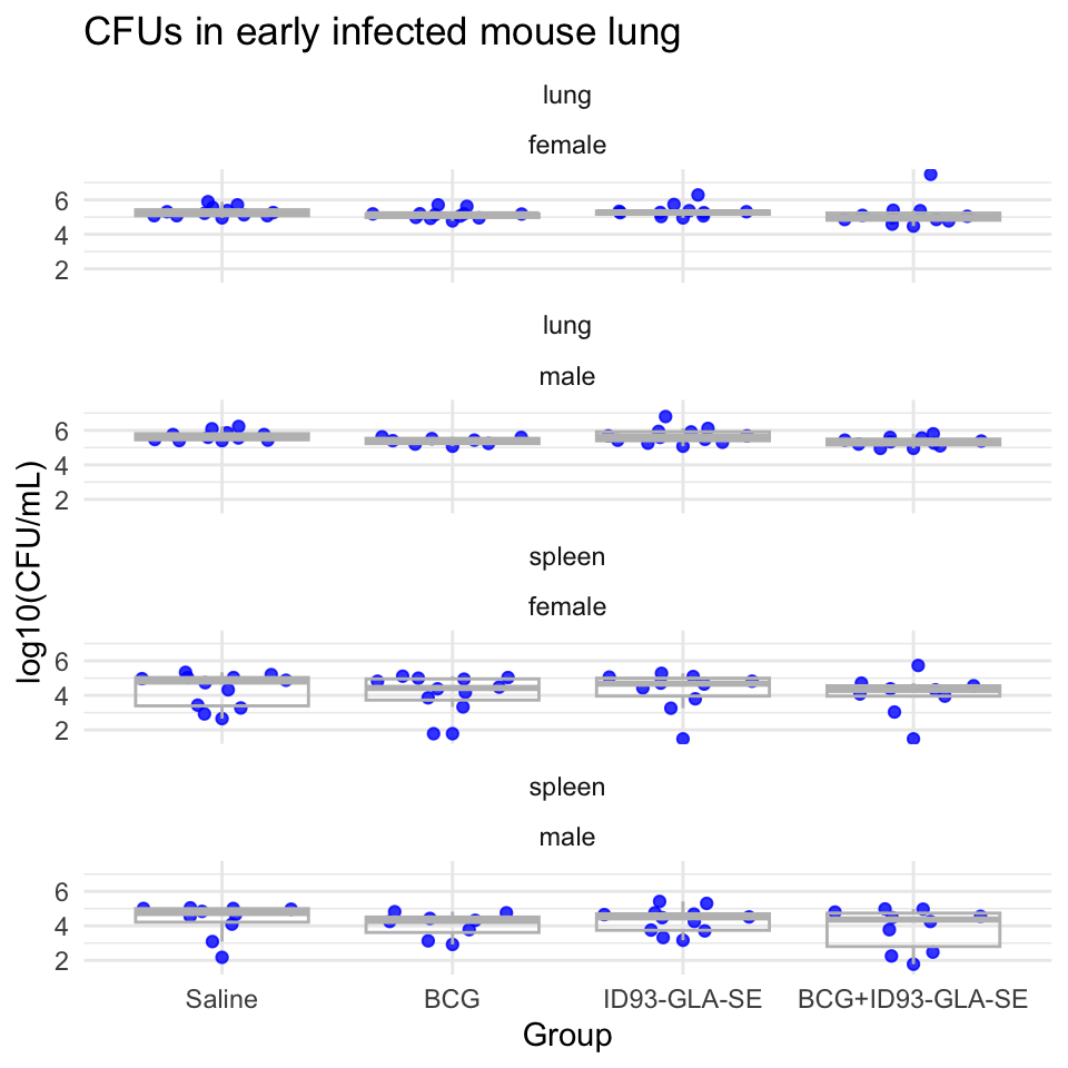
Next, the pipeline creates a plot showing the distribution of CFUs by experimental group in each of the organs:
Next, the pipeline runs an ANOVA analysis on the data. This is conducted after transforming the CFUs with a log-10 transform.
| organ | contrast1 | contrast2 | estimate | conf.low | conf.high | adj.p.value |
|---|---|---|---|---|---|---|
| lung | BCG | Saline | -0.2368058 | -0.5832132 | 0.1096016 | 0.2844430 |
| lung | ID93 GLA SE | Saline | 0.0407358 | -0.2933692 | 0.3748408 | 0.9886291 |
| lung | BCG+ID93 GLA SE | Saline | -0.2381384 | -0.5760187 | 0.0997419 | 0.2587702 |
| lung | ID93 GLA SE | BCG | 0.2775416 | -0.0688658 | 0.6239490 | 0.1614924 |
| lung | BCG+ID93 GLA SE | BCG | -0.0013326 | -0.3513826 | 0.3487175 | 0.9999996 |
| lung | BCG+ID93 GLA SE | ID93 GLA SE | -0.2788742 | -0.6167545 | 0.0590061 | 0.1420190 |
| spleen | BCG | Saline | -0.2738479 | -1.0919602 | 0.5442645 | 0.8159594 |
| spleen | ID93 GLA SE | Saline | -0.0292823 | -0.8276782 | 0.7691136 | 0.9996778 |
| spleen | BCG+ID93 GLA SE | Saline | -0.4036624 | -1.2329754 | 0.4256505 | 0.5798709 |
| spleen | ID93 GLA SE | BCG | 0.2445656 | -0.5735467 | 1.0626780 | 0.8612381 |
| spleen | BCG+ID93 GLA SE | BCG | -0.1298145 | -0.9781256 | 0.7184965 | 0.9779295 |
| spleen | BCG+ID93 GLA SE | ID93 GLA SE | -0.3743802 | -1.2036931 | 0.4549328 | 0.6381738 |
## [1] 0.6506753## [1] 0.8720107## [1] 0.3555729## [1] 0.01680341## [1] 0.2140449## [1] 0.0267285As a last step, the code in the template writes a CSV file with the processed data. This file will be an input into a script that will format the data to add to a database where we are collecting and integrating data from all the CSU experiments, and ultimately from there into project-wide storage.